Investing in Russia: a cross country comparison

As an investor, I have some emergent market bonds, and thus, I am highly interested in the performance of the countries in this category.  As a Russian, I always prefer to know more about its potential relative to other countries.  Below are several simple graphs showing the growth of GDP per capita in absolute and relative terms.   Per head values say more about actual potential not related to population fluctuations.

I compare Russia to four different country groups: China and India; countries from the former USSR; East European countries (former socialist countries); a few Asian countries. There are three time points of interest: 1991 (the start of transition period), 2001 (the start of sustainable growth as a capitalist country), and 2008 (the peak before the current crises). Therefore, I have normalized the GDP per capita time series to their respective values in 1991, 2001, and 2008. The normalized curves illustrate the evolution of the corresponding economies in relative terms. Figures 1 through 4 display the obtained result for four country groups (Russia is always shown by a black line).  All data are borrowed from the Total Economy Database(TED) compiled by the Conference Board (as of October 5, 2012).  The GDP per capita figures are in 2011 US$ converted to 2011 price levels with updated 2005 EKS PPPs.

There are several conclusions from the graphs:

1.       Since 1991, India and China have been doing better than Russia in relative terms but still lag behind the Russian level of GDP per capita.  Since 2001, India and Russia are close with China opening a larger gap.  Since 2008, the Russian economy has been falling apart. Hopefully, the negative deviation is an indication of a higher rate associated with a recovery growth in the near future. In any case, I am lucky to have the Indian and Chinese bonds in my portfolio together with the Russian ones.

2.       Among Former Soviet countries, Russia is not a good performer as well. It is in the middle of the growth curves since 1991, 2001, and 2008. The level is almost the highest, however.  Hence, Russia is a good representative on average. It is not the best performer, but is less sensitive to the current crisis than many of the FSU countries. Therefore, there is no reason to diversify investments over the FSU countries - one will get the result close to the Russian one.  When investing in the best performers one may meet a higher risk of slow down. The poor performers with a higher recovery potential are also characterized by a higher risk.  

3.         Russia is in the middle of the GDP per capita distribution among East European countries. It has been growing slowly since 1991, but outperformed almost all countries since 2001. As mentioned above, Russia was very sensitive to the 2008 crisis and the GDP per capita fell by 9%. It is one of the worst performances among East European countries. The rate of recovery since 2009 is the highest, however. If continued to intersect the paths of Poland and Albania, this recovery growth may bring a fortune for an investor.  

4.       Among Asian countries, Russia is a good performer since 2001, but the poorest one since 2008.

Figure 1. The level of GDP per capita (upper panel) and the evolution of GDP per capita normalized to 1991, 2001, and 2008. The case of India, China and Russia. 

 

Figure 2. The level of GDP per capita (upper panel) and the evolution of GDP per capita normalized to 1991, 2001, and 2008. The case of the countries from the former USSR.

Figure 3. The level of GDP per capita (upper panel) and the evolution of GDP per capita normalized to 1991, 2001, and 2008. The case of the East European countries.

Figure 4. The level of GDP per capita (upper panel) and the evolution of GDP per capita normalized to 1991, 2001, and 2008. The case of the selected Asian countries.

Real GDP per capita since 1870

We've just finished and published a working paper. The reader may want to download it from the MPRA: Real GDP per capita since 1870

Abstract

The growth rate of real GDP per capita in the biggest OECD countries is represented as a sum of two components – a steadily decreasing trend and fluctuations related to the change in some specific age population. The long term trend in the growth rate is modelled by an inverse function of real GDP per capita with a constant numerator. This numerator is equivalent to a constant annual increment of real GDP per capita. For the most advanced economies, the GDP estimates between 1950 and 2007 have shown very weak and statistically insignificant linear trends (both positive and negative) in the annual increment. The fluctuations around relevant mean increments are characterized by practically normal distribution. For many countries, there exist historical estimates of real GDP since 1870. These estimates extend the time span of our analysis together with a few new estimates from 2008 to 2011.  There are severe structural breaks in the corresponding time series between 1940 and 1950, with the slope of linear regression increasing by a factor of 4.0 (Switzerland) to 22.1 (Spain). Therefore, the GDP estimates before 1940 and after 1950 have been analysed separately. All findings of the original study are validated by the newly available data. The most important is that all slopes (except that for Australia after 1950)  of the regression lines obtained for the annual increments of real GDP per capita are small and statistically insignificant, i.e. one cannot reject the null hypothesis of a zero slope and thus constant increment. Hence the growth in real GDP per capita is a linear one since 1870 with a break in slope between 1940 and 1950.  

Key words: GDP, model, economic growth, inertia, trend, OECD

Why the Economic Projections of Federal Reserve Board are inconsistent

The FRB members have recently projected the evolution of key macroeconomic variables including real GDP and the rate of unemployment. In our blog , we have developed a very accurate model linking the rate of unemployment in the US to the rate of real GDP (per capita) growth: (A series of posts has resulted in a working paper.) The following relationship was estimated:

du = -0.62dlnG + 1.09,  (1)

When integrated between t0 and t, equation (1) can be rewritten in the following form:

u(t) = u(t0) + bln[G/G0] +a(t-t0) + c  (2)

Without loss of generality, we assume t0=0. The intercept c≡0, as is clear for t=t0. Instead of integrating (2), we calculate cumulative sums of the annual estimates of du and lnG with appropriate initial conditions. The cumulative sum of du’s is the time series of the unemployment rate. Figure 1 depicts the measured and observed curves for the period between 1958 and 2011. The agreement is excellent and has been obtained by a formal statistical method (LSQR).

 From (1) it follows that higher rates of GDP growth decrease the rate of unemployment. The FRB has projected real GDP with the highest rates of 2.7% in 2012, 3.2% in 2013, and 4% in 2014. We reduce these rates by 1% per year to estimate the per capita rate of growth, i.e. the growth in population is 1% per year. Using (2) we calculate the rate of uneployment which will correspond to the projected real GDP.

Figure 1 also depicts these predicted rates for 2012 to 2014 by open circles. The rates of unemployment projected by the FRB are shown by red circles. There is a significant deviation between the predicted and projected rates, which likely manifests the inconsistency in the FRB member's models of unemployment.

One may check these projections in 2015. 

Figure 1. The observed and predicted rate of unemployment in the USA between 1958 and 2010.The projected rate of unemployment (middle point of the projections) is shown by red circles. 

Tim Duy on Japan or why macroeconomics is wrong

Tim Duy on Economists View posted (http://economistsview.typepad.com/economistsview/2012/01/fed-watch-japan-revisited.html) on the current recovery of Japan and also mentioned usuall macroeconomic rubbish on "lost decades". This is one of good examples showing that the mainstream macroeconomic theories are  worthless and confusing. These people do not actually understand what drive a developed economy like the Japanese one.

We have already decribed the evolution of  a developed economy as expressed by real GDP per capita, G. There are two component in play - inertial growth, A/G,  and the change in a specific age population, dNs/Ns ( following paragraph is borrowd from our book "mechanomics. Economics as Classical Mechanics)

dG(t)/G(t)=A/G(t)+0.5dN_s(t)/N_s(t)dt   (1.8)

where A is an empirically determined coefficient, N_s(t) is the number of people of the defining age. For Japan, the defining age of eighteen years has been found.  Relationship (1.8) implies that the growth rate of GDP depends explicitly and entirely on the attained level of real GDP per capita and the population change. If to gather relevant terms on both sides of the equation, this relationship can be simplified in the following form: 

d[G(t)-(At+C)]/G(t)= 0.5dN_s(t)/N_s(t)  (1.9)

where C is the constant of integration, i.e. the initial condition of the initial value problem. 

From (1.9) one can derive either the evolution of G or Ns depending on the purpose. Since the number of 18-year-olds can be estimated by integrating (actually by summation of discrete estimates) the left hand side of (1.9) with the measured annual values of G and also enumerated by population surveys one can  compare results visually and statisticaly. Figure 1.23 (also from the book) demonstartes that the evolution of G follows up the evolution of Ns. Since G can not affect Ns the causality directio is opposite - the change in Ns drives G.   From 1.23, one can  understand that so called "lost decades" actually manifest the fall in the number of 18-year-olds since 1992. Accordingly, the years before 1991 are charaterized by increasing Ns and thus are called "economic  miracle".  Finally, one can extrapolate the younger age cohorts into the future and estimate the future evolution of G. Figure 1.23 shows that the years of low economic growth are left behind and the 2010s will be charaterized inertial growth only, A/G, since Ns will not be changing. This is not fast economic growth, A/G~ 1.5% per year, but is definitely better than the permanent depression of the 1990s and 2000s.

Figure 1.23. Enumerated and predicted number of 18-year-olds.

Some corrections to David Altig's job market charts

David Altig presented some projections of the unemployment rate based on various monthly increments in employment.  It was a crude estimate because it did not include inherent fluctuations in the growth of working age population and labor force participation rate. It is much better to use Okun’s law linking unemployment and the real GDP growth.

Previously in this blog, we presented a version of Okun’s law for the rate of unemployment in the USA since 1955 as defined by real GDP per capita. We have estimated Okun’s law coefficients in two different segments using a standard LSQ technique. The reason behind the split into two segments was the change in realGDP estimation procedure introduced around 1978 - the definition of the GDP deflator was dramatically changed. We discussed this important methodical issuein our blog.

The best-fit (dynamic) model minimizing the RMS error of the cumulative model is as follows:

du = -0.406dlnG + 1.113, t<1979

du = -0.465dlnG + 0.866, t>1978 

This model suggests a smaller shift in the slope and a larger change in the intercept around 1979. This Okun’s law is characterized by a standard error of 0.53% for the period between 1958 and 2010. The average rate of unemployment for the same period is 5.6% with an average annual increment of 1.06%.

            Using the relationship for the period after 1979, one can estimate the evolution of the unemployment rate for various growth rates o real GDP per capita. We have selected three different values: 1% per year, 1.86% per year, and 3% per year. The first value is approximately equal to the mean growth rate between 2000 and 2010 (11 years) which is 0.93% per year. The second value provides a constant rate of unemployment, as defined by the ratio of coefficients 0.866/0.465 and is slightly higher than the mean rate after 1980 (1.63% per year). The third value is very high and just demonstrates the condition to reduce the rate of unemployment to 4% by 2020.  Figure 1 depicts the predicted and observed rate of unemployment after 1980 and these three projections. This is a more accurate projection than that by David Altig.

I do not see any opportunity for the rate of unemployment to fall any time soon. In the long run, unemployment will remain high. For the slow growth scenario expected by the FRB, u may reach 13% by 2020.

 Figure 1. Observed, predicted and projected rate of unemployment in the USA.

Revised GDP estimates support the model of inertial growth

On July 29, the BEA revised real GDP estimates for the years after 2007. The most important news is:

For 2007-2010, real GDP decreased at an average annual rate of 0.3 percent; in the previously 

published estimates, real GDP had increased at an average annual rate of less than 0.1 percent. From the fourth quarter of 2007 to the first quarter of 2011, real GDP decreased at an average annual rate of 0.2 percent; in the previously published estimates, real GDP had increased at an average annual rate of 0.2 percent. 

These new BEA data strongly support our model of real economic growth. Previously in this blog, we found that real GDP per capita in developed countries grows as a linear function of time. Similarly to classical mechanics, we interpret this linear growth as “inertial” growth. When the population pyramid does not change over time one can write the following relationship for real GDP per capita, G(t):

G(t) = At + C           (1)

Relationship (1) defines the linear trajectory of the GDP per capita, where C=G_i(t₀)=G(t₀) and t₀ is the starting time. In the regime of inertial growth, the real GDP per capita increases by the constant value A per time unit. Figure 1 depicts the evolution of annual increment of real GDP per capita in the U.S. since 1950. The new GDP revision makes the slope of the linear regression line (trend) almost negligible (+$1.9 per year) and thus supports our concept. In 2011, the slope may become negative if the increment is below $432. After the two mediocre quarters in 2011, we would not expect real GDP per capita in 2011 to grow faster than in 2010.  

On June 5 we had a post on the current position of the U.S. economy relative to some long term trend. As a rule, economists consider real growth as an exponential process and see the U.S. economy far below its trend. We compared the trends in real GDP and GDP per capita. The latter should be a linear one. Figure 2 depicts the evolution of both variables between 1950 and 2010 with the new readings between 2007 and 2010.

The real GDP curve has an exponential shape as related to the growth in total population. One can easily observe the current deviation from the exponential trend and blame poor economic conditions after 2007. With the decelerating rate of total population growth we would not expect the observed curve to return to the exponential trend (exponential extrapolation of the previous growth.)  

The real GDP per capita evolves along a straight line. After the revision, the curve falls below the linear trend. It touched the trend with the previous set of GDP estimates. All in all, during the past four years the observed curve returned to the long-term trend and may stay below the trend for a while.   We also presented an exponential trend which has a small coefficient of 0.02. This coefficient effectively makes the line very close to a straight one between 1 and 60. However, the deviation from the (extrapolated) exponential trend will be growing and observations will contradict the hypothesis of exponential growth. 

Figure 1. Annual increment of real GDP per capita in the U.S. between 1950 and 2010.

Figure 2. The evolution of real GDP and real GDP per capita between 1950 and 2010. 

Okun's law integrated: France

We have just estimated a version of Okun’s law for the USA. We have applied a LSQ technique to the integral version of Okun’s law:

u(t) = u(t0) + bln[G/G0] + a(t-t0) (1)

where u(t) is the rate of unemployment at time t, G is the level of real GDP per capita, a and b are empirical coefficients.

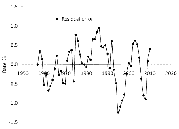
For France, we have a model estimated by a simple eye-fit. Here we re-estimate the model  with a structural break somewhere between 1980 and 1990. The best-fit (dynamic) model minimizing the RMS error of the cumulative model (1) is as follows:

du = -0.155dlnG + 0.805, t<1987

du = -0.508dlnG + 0.710, t>1986 (2)

This model suggests a big shift in the slope and a smaller change in the intercept around 1986. Figure 1 depicts the observed and predicted curves. The agreement is very good, with the highest difference since 1995 which might be associated with the change in monetary policy.

The cumulative form of the dynamic Okun’s law is characterized by standard error of 0.60% for the period between 1958 and 2010. The average rate of unemployment for the same period is 3.3% with an average annual increment of 0.59%. Figure 2 displays the cumulative model error.

Figure 1. The observed and predicted rate of unemployment in the France between 1962 and 2010.

Figure 2. The residual error or the cumulative model.

Okun's law integrated

In our previous post, we have estimated Okun’s law for the USA and several develop countries. This law links real economic growth and the change in unemployment rate. Here we integrate this relationship and obtain the dependence of the unemployment rate on real GDP. It allows modeling the rate of unemployment over time.

We have rewritten Okun’s law using the growth rate of real GDP per capita instead of GDP itself:

du = a + bdlnG (1)

where du is the annual increment in the rate of unemployment, dlnG=dG/G is the relative change rate of real GDP per capita per one year, a and b are empirical coefficients. Okun’s law suggests that b<0.

The reason to use per head values is obvious – the rate of unemployment is a population independent characteristic (i.e. normalized to total population) and GDP implicitly includes the change in population. When the change in population is fluctuating, relationship (1) is biased.

For the United States we have obtained the following relationship:

du = -0.42dlnG + 1.07, t<1985

du = -0.62dlnG + 1.09, t>1984 (2)

with a structural break in 1984. This was a preliminary assessment of the links as based on an eye-fit between measured and predicted curves. No formal minimization was applied.

When integrated between t0 and t, equation (1) can be rewritten in the following form:

u(t) = u(t0) + bln[G/G0] +a(t-t0) + c (3)

Without loss of generality, we assume t0=0. The intercept c≡0, as is clear for t=t0. Instead of integrating (3), we calculate cumulative sums of the annual estimates of du and lnG with appropriate initial conditions. The cumulative sum of du’s is the time series of the unemployment rate. Figure 1 depicts the measured and observed curves. The agreement is excellent and has been obtained by a formal statistical method.

We have re-estimates all coefficients in (3), and thus in (2), using a LSQ technique. Since we have already introduced a structural break in (2), we have sought the best fit allowing the year of this break to vary between 1970 and 1990. The best-fit (dynamic) model minimizing the RMS error of the cumulative model (3) is as follows:

du = -0.406dlnG + 1.113, t<1979

du = -0.465dlnG + 0.866, t>1978 (4)

This model suggests a smaller shift in the slope and a larger change in the intercept around 1979. The break year has changed from 1984 to 1979. This is a very important finding because both relationships in (4) give very close predictions for the period between 1978 and 1985. Therefore, the shift in coefficients in (4) is likely not an abrupt one but actually a transition process between two different states of the US economy.

The cumulative form of the dynamic Okun’s law (4) is characterized by standard error of 0.53% for the period between 1958 and 2010. The average rate of unemployment for the same period is 5.6% with an average annual increment of 1.06%. Figure 2 displays the cumulative model error.

Figure 1. The observed and predicted rate of unemployment in the USA between 1958 and 2010.

Figure 2. The residual error or the cumulative model (4).

Okun’s law revisited. Is there structural unemployment in developed countries?

Abstract

Okun’s law for the biggest developed countries is re-estimated using the most recent data on real GDP per capita and the rate of unemployment. Our results show that the change in unemployment rate can be predicted with a high accuracy. The link needs the introduction of a structural break which might be caused by the change in monetary policy or/and in measurement units. Statistically, the link between the studied variables is characterized by the coefficient of determination between 0.40 (Australia) and 0.84 (the USA). The residual errors can be associated with measurement errors. The obtained results suggest the absence of structural unemployment in the studied developed countries.

Key words: unemployment, GDP, modelling, Okun’s law

JEL classification: J65 

Introduction

The Sveriges Riksbank Prize in Economic Sciences in Memory of Alfred Nobel 2010 was awarded to P. Diamond, D. Mortensen and C. Pissarides ”for their analysis of markets with search frictions”. The core result of their study was an explanation of labour market dynamics including unemployment (e.g. Diamond, 2011; Mortensen and Nagypal, 2007; Pissarides, 2000). Hence, the dynamics of unemployment is a very important and actual problem for the modern economics.

One of the most actively discussed topics related to unemployment is its high persistence since the start of the financial crisis. In the United States, the current rate unemployment is above 9% and it does not show any sign of reduction in the future. There is an opinion that the current situation might manifest tangible structural changes in the labour market. This implies some major changes in the overall organization of the economy when significant parts of it become unnecessary.

We address the problem of structural unemployment by modelling the rate of unemployment using the relationship explaining the dynamics of unemployment by its negative correlation with the growth in GDP – Okun’s law (1962). This relation was revisited many times in the past (e.g. Altig, Fitzgerald and P. Rupert, 1997; Knotek, 2007; Tillman, 2010).

We also revisit Okun’s law using the most recent data on GDP per capita provided by the Conference Board (2011) and data on unemployment from the OECD (2011). To improve the agreement between the change in unemployment rate and real GDP per capita we introduce structural breaks in Okun’s law. Such breaks might manifest artificial changes in definitions of unemployment and real GDP as well as actual shifts in the linear relationship.

We have assessed Okun’s law in the biggest developed countries: the United States, France, the United Kingdom, Australia, Canada and Spain. Our results suggest the absence of structural unemployment in the studied developed countries. The persistence of high unemployment is completely related to low rate of real economic growth. In all studied countries, the rate of growth above 2% per year will result in a fall of the unemployment rate.

Okun’s law and empirical results

According to the original form of Okun’s law, there exists a negative relation between the growth rate of real GDP and the change in unemployment rate, du=u_i-u_i-1. The overall GDP includes the change in population as an extensive component which is not necessary dependent on other macroeconomic variables. Econometrically, it is mandatory to use macroeconomic variables of the same origin and we use real GDP per capita, G. It is better related to the portion of labor force without job, i.e. the rate of unemployment. Therefore, we rewrite Okun’s law in the following form:

            du = a + bdlnG      (1)

where dlnG=dG/G is the relative change rate of real GDP per capita, a and b are empirical coefficients.  Okun’s law suggests that b<0.  

We start with the United States and have to introduce a structural break in 1984 into the link. The following relationship was obtained:  

 du = -0.42dlnG + 1.07, t<1985

 du = -0.62dlnG + 1.09, t>1984             (2) 

where dlnG in the annual growth rate of real GDP per capita, du is the annual increment in the rate of unemployment, u. Figure 1 displays the observed and predicted du between 1958 and 2010. The agreement is excellent. Figure 2 presents some regression results for the curves in Figure 1 with the coefficient of determination R²=0.84. Therefore, more than 84% of the variability in the change of unemployment rate in the U.S. is explained by the change in real GDP per capita. Considering the fact that both macroeconomic variables are measured with an accuracy of approximately 1 percentage point the residual 16% of the variability can be easily associated with the uncertainty in their measurements. Figure 3 demonstrates that the residual error is rather random and does not contain a unit root and has no significant autocorrelation.

Relationship (2) shows that the sensitivity of the du to dlnG becomes higher after 1984 with the slope of -0.62 and the intercept +1.09. There are two assumptions on the reasons behind this structural break. One is related to the changes in monetary policy in the early 1980s to overcome extremely high inflation. On the other hand, the measures of the GDP deflator and CPI start to deviate around 1980 and the rate of unemployment obtained a new definition in 1984. Thus, the shift in 1984 might also be associated with new units of measurements. In any case, the period after 1984 is described with a very high accuracy including three episodes of unemployment surge in 1991, 2001 and 2009. Moreover, relationship (2) provides a smooth transition through 1984 and describes the fall in unemployment in 1984.

We have also checked several macroeconomic variables as a predictor variable in Okun’s law: the overall GDP, GDP per capita corrected for the difference between the whole population and working age population, and productivity as expressed by real GDP per worker.  All these variables are inferior to real GDP per capita and thus we use this variable for other countries.

The next country to model is France. We have reversed (1) and obtained the following relationship for dlnG:  

 dlnG = -5.0du + 4.6, t<1987

 dlnG = -1.5du + 1.4, t>1986                      (3)

Figure 4 present the observed and predicted curves. There is a shift in the dependence around 1987 and the slope in (3) fell from -5.0 to -1.5.  Correspondingly, the sensitivity of the unemployment rate to real GDP growth (the reciprocal value of the slope in (3)) increased from -0.2 to -0.67. In order to decrease the rate of unemployment in France, real GDP per capita has to grow by 1.5% per year. When the growth rate is lower, the rate of unemployment increases. 

For France, both variables are characterized by an elevated volatility and thus the coefficient of determination R²=0.53 is relatively low. To remove the measurement noise we have smoothed both curves with MA(3). The lower panel in Figure 4 shows that the agreement between the measured increase in real GDP per capita and that predicted from the change in unemployment rate became extremely good.  

The United Kingdom also shows an excellent result for Okun’s law. The following equation:

dlnG = -1.5du + 2.5, t<1987

dlnG = -2.0du + 1.7, t>1986                 (4) 

describes the period after 1972. Figure 5 illustrates the agreement between the observed and predicted time series. Before 1972, the OECD provides no unemployment estimates. The year of structural break is the same as in France but the change in the slope is much lower. In any case, to reduce the current rate of unemployment the UK needs to grow at a rate above 1.7% per year in term of real GDP per capita.  

For Canada, the following equation was estimated with a structural break around 1985:  

dlnG = -2.7du + 3.1, t<1985

dlnG = -2.7du + 1.2, t>1984       (5) 

Figure 6 depicts the measured and predicted curves for dlnG. For Canada, the rate of growth above 1.2% per year is enough to reduce the rate of unemployment from its current level of 8%. In 2009, dlnG=-0.033 y^-1 and the rate of unemployment rose by 4.7%. In 2010, the change rate of real GDP per capita was +0.021y^-1 and the rate of unemployment fell by 0.3%.   For Australia, the following equation was estimated with a structural break around 1995:  

dlnG = -1.7du + 2.4, t<1995

dlnG = -3.0du + 1.2, t>1994       (6) 

The timing of this break is different from those obtained before but the shift in the slope and intercept is big enough to consider it with confidence. It is likely that the structural break was induced by the introduction of a new monetary policy in 1994 (RBA, 1994).

 

Figure 1.  The link between the du and dlnG in the U.S. as described by relationship (2) with a structural break in 1984 

Figure 7 displays the measured and predicted curves for dlnG. The overall agreement is not good with R²=0.40 for the period between 1968 and 2010. This low correlation coefficient is associated with the high volatility in both time series. When smoothed with MA(3), the curves in Figure 7 show a much better resemblance. For Australia, the rate of growth above 1.2% per year is enough to reduce the rate of unemployment from its current level of 5.2% (2010). It is similar to Canada. 

Finally, the case of Spain is a decisive one. The rate of unemployment in Spain is extremely high and has been varying in a wider range since the 1960s. This is a big challenge for Okun’s law. We have obtained the following relationship with a structural break in 1987:  

dlnG = -2.0du + 5.0, t<1987

dlnG = -0.8du + 2.1, t>1986                     (7) 

The timing of this break practically coincides with those in other countries. The sensitivity of unemployment to real economic growth rose significantly in 1987. 

Figure 8 displays the measured and predicted curves for dlnG. The overall agreement is not good with R²=0.59 for the period between 1961 and 2010. When smoothed with MA(3), the curves in Figure 8 show an extraordinary agreement but one can also introduce another structural break near 1968.

Figure 2.  A scatter plot du against dlnG from Figure 1with a linear regression line. R²=0.84.

Figure 3. The model error for the U.S.

Figure 4.  Observed and predicted dlnG for France. The lower panel presents the curves smoothed with MA(3).

Figure 5.  Observed and predicted dlnG for the UK. The lower panel presents the curves smoothed with MA(3). 

Figure 6.  Observed and predicted dlnG in Canada. The lower panel presents the curves smoothed with MA(3).

Figure 7.  Observed and predicted dlnG in Australia. The lower panel presents the curves smoothed with MA(3).

Figure 8.  Observed and predicted dlnG in Spain. The lower panel presents the curves smoothed with MA(3).

Conclusion

With real GDP per capita instead of the overall GDP, Okun’s law demonstrates an extraordinary predictive power for the biggest developed countries. One can accurately describe the dynamics of unemployment since the 1960s. The currently high levels of unemployment in developed countries cannot be reduced without fast economic growth well above 2% per year. In that sense, there are no structural unemployment components in the currently high rates of unemployment in the studied countries. 

References

Altig, D., T. Fitzgerald, and P. Rupert. (1997). Okun’s Law Revisited: Should We Worry About Low Unemployment?” Federal Reserve Bank of Cleveland, Economic Commentary.

Conference Board. (2011).  Total economy database. http://www.conference-board.org/data/economydatabase/

Diamond, P. (2011). Unemployment, Vacancies, Wages. American Economic Review, 101(4): 1045–72.

Knotek, E. S. II. (2007). How Useful is Okun’s Law?, Federal Reserve Bank of Kansas City Economic Review, 4th Quarter, 73-103.

Mortensen, D. T. and E. Nagypal. (2007). More on Unemployment and Vacancy Fluctuations, Review of Economic Dynamics, 10 (3): 327{347.

Okun, A. M. (1962). Potential GNP: Its Measurement and Significance, American Statistical Association, Proceedings of the Business and Economics Statistics Section, 98–104.

Organization of Economic Cooperation and Development (2011). Original release data and revisions database. http://stats.oecd.org/mei/default.asp?rev=1

Pissarides, C. A. (2000). Equilibrium Unemployment Theory, Cambridge: MIT.

Reserve Bank of Australia. (1994). 1994 Report and Financial Statements. Reserve Bank of Australia. Sydney

Tillmann,  P. (2010). Do FOMC members believe in Okun's Law? Economics Bulletin,  30, No. 3, 2398-2404.