In the Solow growth model, the rate of change in real GDP per capita must approach some constant level. This is a result of the following assumption: labor and knowledge grow at constant rates and the rate of capital growth is proportional to the level of output and the rate of capital depreciation. All assumptions are taken without empirical justification. However, actual data on real GDP tell a different story.
Under the empirical framework we presented in this blog, real GDP per capita in developed countries grows as a linear function of time, we call it inertial growth, when population pyramid does not change much in the long run:
G(t)=At+C (1)
Relationship (1) defines the linear trajectory of the GDP per capita, where C=Gi(t0)=G(t0) and t0 is the starting time. In the regime of inertial growth, the real GDP per capita increases by the constant value A per time unit. The relative rate of growth along the inertial linear growth trend, g(t), is the reciprocal function of G:
g(t)= A/G(t) (2)
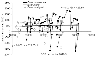
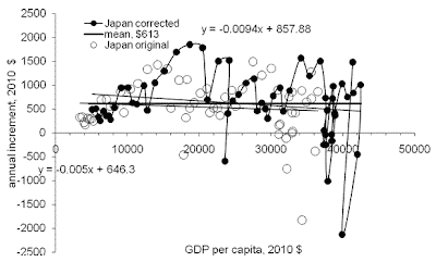
Relationship (2) implies that the rate of GDP growth will be asymptotically approaching zero, but the annual increment A will always be constant. This is different from the Solow model where the rate of growth is a positive (nonzero) value. Moreover, the absolute rate of GDP growth is constant and is equal to A [$/y]. This constant annual increment thus defines the constant “speed” of economic growth in a one-to-one analogy with Newton’s first law. Hence, one can consider the property of constant speed of real economic growth as “inertia of economic growth” or simply “inertia”. In Figure 1, we present annual increments of real GDP per capita (borrowed from the Conference Board Total Economic database) in the biggest developed economies as a function of real GDP per capita in sense of equation (1). These plots validate our empirical finding and reject the Solow model. Overall, there were 19 countries analyzed in the study and no one has any distinct positive trend over the past 60 years, i.e. between 1950 and 2010.
In Figure 1, the original GDP time series are extended by those corrected for the ratio of total and working age population (the latter must be used in GDP per capita calculations). For both time series linear regression lines and equations are shown with corresponding slopes. For the biggest countries these slopes are very close to zero but can be positive or negative. A zero slope corresponds to constant annual increment.
So, we have 1000 years validating the hypothesis of a constant (but country dependent) annual increment.
Figure 1. Dependence of annual GDP increment on GDP (both real per capita) for select developed countries. Original GDP data are extended by those corrected for the ratio of total and working age population (the latter must be used in GDP per capita calculations). For both time series linear regression lines and equations are shown with corresponding slopes. For the biggest countries these slopes are very close to zero but can be positive or negative. A zero slope corresponds to constant annual increment.


0 komentar:
Post a Comment