Lillie and Walter

Lillie and Walter are my great-grandparents. They were married on the 26th of  November 1913 in the Salt Lake Temple.  Here is one of their wedding pictures:

(Aside: I first saw this photograph a few years ago and was fascinated by it.  They both look so young.  And BTW, I am so glad that we have the technology that allows us to share and copy so easily things like photos.  I doubt whether I would have ever seen the photo without digital scanning technology that lets me have my own copy.)

They look so serious in the photos, but I like to think they were an idyllic couple, and I don't have any reason to doubt that they were.


Lillie was of Swedish extraction (surname Fernelius) and Walter was of Welsh (surname James) extraction.  They had one child, a daughter, named Afton, my paternal grandmother.

 Lillie (on the left) before her marriage (with sister Ellen in the middle and a friend on the right. Pay no attention to the wastebaskets on their heads)

 Walter before his marriage

My grandmother, Afton, was their only child because tragedy struck early in their marriage.  My great grandfather was killed in a hunting accident on 1 September 1915 in Mountain Green, Utah.  Afton, born on 17 January 1915, was only nine months old when her father died.


After Walter died, Lillie and Afton left Evanston, Wyoming where Walter had worked for the Union Pacific Railroad as a fireman (shoveling coal into the firebox of the locomotive) and returned to South Weber to live with her parents.

Lillie eventually remarried a few years later (October 6, 1920) to a widower named Charles Hunt, who had two young children (Charles and Bernice).  He had lost his wife in the Spanish Flu epidemic of 1918.

Since Lillie and Walter were married for time and eternity in the Salt Lake temple by the authority of the priesthood and with the sealing power of Elijah, I believe that they are together as husband and wife in heaven.

Members of the Church of Jesus Christ of Latter Day Saints believe that families can be eternal through covenants made in temples, just like the one being built right here in Brigham City

Lillie and Afton

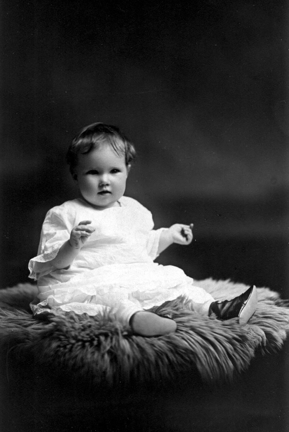
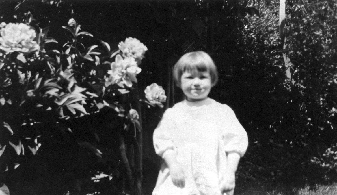
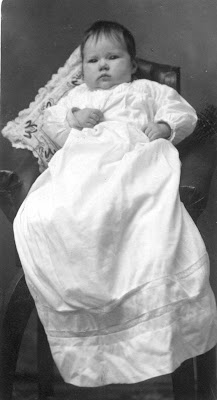
Pictures of Afton as an infant and child:

GeoResources is highly overvalued

We have just discussed in our previous article the price evolution of Newfield Exploration Company and found that its current share price is highly undervalued relative to the fundamental price level.  The latter is defined by our pricing model based on share price decomposition into a weighted sum of individual consumer price indices (alternatively PPIs). Here we present an opposite case – GeoResources (NYSE: GEOI), an independent oil and gas company, which engages in the acquisition, re-engineering, development, and exploration of oil and gas reserves in the Southwest, Gulf Coast, and the Williston Basin areas of the United States. This company with capitalization of ~$850M is highly overvalued relative to the predicted (fundamental) price.

Our pricing concept and approach have been discussed many times. For example, articles [1, 2, 3] were devoted to ConocoPhillips (NYSE: COP), which provides an excellent benchmark  and general explanation of the quantitative definition of fundamental price.  The measured COP price is accurately described by a linear combination of two consumer price indices, the core and headline ones. The headline CPI plays the role of that part of the overall energy price which is directly related to the share price.  The agreement is so good that it is difficult to deny that energy (in one form or another) drives the evolution of ConocoPhillips.

The best fit (LSQ) model for GEOI share is the following:

GEOI(t) = -2.59CC(t-0) + 0.14E(t-0) + 11.63(t-2000) + 321.12 ; sterr=$2.87

where GEOI(t) is the share price in U.S. dollars at time t, CC is the core CPI, and E is the consumer price index of energy.   The model standard error is only $2.87 for the period between July 2003 and March 2012. The model also allows both CPIs to lead the share price by 0 to 12 months. However, the best lags are both zero. The index of energy drives the price up, and the core CPI affects the price negatively. Figures 1 and 2 depict the observed and predicted monthly prices and the residual model error, respectively.  

The overall agreement is good but the model residual has several spikes; the most recent has been observed since the second half of 2011. Currently, the error is +$6.5, which is an extremely high residual for GEOI. The same positive residual was observed a year ago. It had returned quickly to the predicted curve and then was followed by a negative residual of approximately the same amplitude. Therefore, the evolution of GEOI price is characterized by very high volatility likely associated with its size; smaller companies are subject to higher risks.  At the same time, the COP model proves that the predicted price might play the role of “fundamental” price. Since GEOI is much smaller than COP, one can consider the current positive excursion as a short-term deviation. Then the GEOI price is highly overvalued.

Thus, we expect the GEOI price to fall to the level of $25 per share in the near future, i.e. we expect GEOI to return to its fundamental price.

Figure 1. The observed and predicted monthly closing prices for GEOI between July 2003 and March 2012.

Figure 2. The model residual error. 

Chicken Drummettes Shaken in Thai Sauce

 Few days ago my third son watched the Astro food channel TLP showing chicken drummetts shaken in various choices of sauce sold in USA restaurant chain. He was really drooling and asked me to try making them. So here is my own simple creation of the sauce.... I placed the sauce in a container (like what shown in the tv) and add in fried chicken.... shaked it until well coated and ready.... My son was satisfied with the outcome!

 

By: Roz@HomeKreation
Serves: 4-5 persons
INGREDIENTS:
10 Chicken Wing Drummettes
1/4 cup Thai Chili Sauce
1/4 cup Chili Sauce
1 tsp Sweet Soy Sauce
2 tsp Honey
Salt & Pepper
Sesame Seeds - fried in some oil 

METHOD:
1. Rub chicken drummettes with salt & pepper.
Deep fry until just cooked but need not be crispy, let it be soft & juicy.
2. Mix the three sauces, honey & sesame seeds in a container.
Add in fried chicken, cover & shake until chicken is well coated with sauce.
3. Serve right away.
***********************************

BAHASA MALAYSIA VERSION

 Idea nak buat ni dari anak Along yg suka tengok food channel kat Astro. Untuk sos tu, Along reka2 jer lah, sedap pula. Senang, tak payah nak teruk2 nak masak bagai, goncang2 dalam bekas dah siap!

By: AlongRoz@HomeKreation

Serves: 4-5 orang

BAHAN2:

10 ketul Kepak Ayam (belah bawah)

1/4 cwn Sos Cili Thai

1/4 cwn Sos Cili

1 st Kicap Manis

2 st Madu

Garam & Lada Sulah

Biji Lenga - goreng sebentar dlm minyak & tapis 

CARA2:

1. Gaul ayam dgn garam & lada.

Goreng sehingga masak, jgn sampai garing supaya ayam tetap lembut.

2. Campurkan ketiga2 sos, madu & biji lenga dalam bekas yg bertutup.

Masukkan ayam & goncang sehingga bergaul rata.

3. Hidangkan segera. Sedap untuk ratah2 atau di hidangkan dgn nasi.

Sauce ingredients that I used

The container that I used to shake the sauce & drummettes

Newfield Exploration Company is highly undervalued

In our previous articles on the Seeking Alpha [1, 2, 3] we demonstrated that the evolution of ConocoPhillips (NYSE: COP) share price can be accurately described by a model based on the share price decomposition into a weighted sum of individual consumer price indices (alternatively PPIs). Both defining CPIs (PPIs) may lag behind the price. This model has been working since 1982 with one structural break around 1998 [2]. This break was related to the change in the long term trend of the difference between the core and headline CPIs [4].

Figure 1 reproduces the observed and predicted COP prices in order to demonstrate the predictive power of the pricing concept. In Figure 2, we depict the model error between 1998 and 2012. One can see that the cumulative model error approached the zero line, i.e. the regression line coincides with the zero line. In other words, all deviations of the actual price from the predicted one are only short-term and the predicted curve might be considered as a “fundamental” one. For ConocoPhillips, we have estimated the following relationships to minimize the model error between 1998 and 2012:

COP(t) = 72.3 – 5.35(CC(t) - C(t))  (1)

where COP(t) is the share price in U.S. dollars at time t, CC(t) is the core CPI, and C(t) is the headline CPI. This relationship is slightly different from that in [2] where we did not minimized the model error.

Figure 1. Historic (monthly closing) prices for COP (black line) and the scaled difference between the core CPI and the headline CPI (red line). 

Figure 2. The model error for COP. The regression line shows that the cumulative error approaches the zero line.

There is a good reason why we discuss the price model for COP over and over. It provides a good benchmark when we estimate quantitative models for different companies.  With the predicted and measured COP prices in Figure 1, it is difficult to deny that energy (in one form or another) drives the evolution of ConocoPhillips. To many readers and/or investors this thought might be a trivial and obvious one. However, the thought that CPI components can drive share prices is not so trivial when we describe the prices of companies from different sectors and industries (e.g. BAC from Financial). The very same approach is treated as an inappropriate one.

In any case, there is no strong criticism of our models for energy related companies we continue presenting them with the case of Newfield Exploration Company (NYSE: NFX),  an independent energy company, engaged in the exploration, development, and production of crude oil, natural gas, and natural gas liquids. As for many other companies, we tested two principal pairs of CPIs: C and CC; CC and the index of energy, E, as well as the pair the PPI and the producer price index of crude oil, OIL. The best fit (we used the LSQ technique) model is obtained with the pair CC and E:

NFX(t) = -4.45CC(t-1) + 0.40E(t-0) + 17.48(t-2000) + 587.71 ; sterr=$7.18  (2)

where NFX(t) is the share price in U.S. dollars. We allowed both time lags (CPI leads the price) in (2) to vary between 0 and 12 months. However, the best lags are one and zero months, respectively. The index of energy drives the price up, and the core CPI affects the price negatively. Figures 3 and 4 depict the observed and predicted monthly prices and the residual model error, respectively.  

The overall agreement is not good when compared to that for ConocoPhillips. Moreover, the model residual has been growing since the second half of 2011. Currently, the error is -$24.4, which is an extremely high residual. Now it’s time to use the COP model as a reference. In line with the interpretation of the COP model error, one might consider the predicted NFX price as a “fundamental” price. Since NFX is much smaller than COP its price is subject to higher fluctuations. Accordingly, the current excursion is just a short-term deviation. Then the NFX price is highly undervalued.

As an alternative explanation, one may suggest that the model has failed on NFX. We cannot exclude this explanation but then why the concept works for the biggest energy companies and has also been working relatively well before August 2011?  Thus, we expect the NFX price to rise to the level of $60 per share in the near future, i.e. to return to its fundamental price. 

Figure 3. The observed and predicted monthly closing prices for NFX between July 2003 and |March 2012.

Figure 4. The model residual error. 

There is another interesting question why do the other two pairs of defining indices have larger residual errors? Obviously, all three oil related indices, i.e. the headline CPI, the index of energy and the producer price index of oil, are tightly linked but are also affected by different goods and services included in the CC and E. The evolution of these defining indices differs accordingly. On the other hand, there is some true set of goods and services which do define the evolution of the NFX price. Then the intercept of this true set and those comprising the CC, E, and OIL should mimic the behavior of the true defining set.   In other words, all three studied indices are just proxy to the true one. As a result, their predictive power may vary with time.

Recording of webinar on using data in an upper division class now available!

The second in a series of webinars on integrating quantitative data analysis into substantive undergraduate social science courses is available for viewing.

Hosted by ICPSR and the Social Science Data Analysis Network (SSDAN), the webinar featured Dr. Rongjun Sun, professor of sociology at Cleveland State University. Jones discussed his tools for helping students measure world income and health inequality. He described his procedures for having his students sort income data in Excel, and calculate the mean incomes and infant mortality rates of the 20 richest and 20 poorest countries in the world.

A video of the presentation is available here (WMV, 45.8 MB), and the accompanying slides are available here (PPT, 125KB).

Persistent URL: http://icpsr.blogspot.com/2012/03/slides-video-from-second-webinar-on.html

Americans Weigh in on the 2010 Health Care Law

March 29^th marks the completion of the final day of the Supreme Court’s health care hearings.  The Court is expected to make its ruling in late June.  In conjunction with the final day of arguments, The New York Times released its polling data on the public’s support and comprehension of the Affordable Care Act and its implications.  The poll finds that 47% of Americans disapprove of the legislation, while 36% approve.  In addition, while the public can only speculate on the outcome of the health care hearings, the American people have specific opinions on how the Supreme Court should handle the case.  26% believe the law should remain intact, 29% favor overturning the individual mandate, and 38% would prefer the Court to find the entire law unconstitutional.  Americans are much more favorable of the law’s specific provisions.  

Aside from the individual mandate (51% of Americans disapprove of the Affordable Care Act’s requirement that Americans purchase health insurance), the majority of Americans support: (1) the Act’s requirement that health insurance companies cover those possessing existing medical conditions, (2) The provision permitting children to remain on their parents’ policies until age 26, and (3) the Affordable Care Act’s attempt to close the prescription drug coverage gap, commonly known as the “doughnut hole.” 

In terms of the personal effects of the 2010 health care law, most Americans believe the legislation will not have much effect on their overall health care benefits or the quality of care they receive, but they do expect their health care costs to increase as a result of the legislation.

Lastly, it appears that many Americans are confused with how the Affordable Care Act will affect them and their families.  48% of the public does not understand the 2,700-page act and the effects it will have on their families, while 47% say they do understand the law.  

Cameron International share price

Following our approach to share pricing of energy companies we present a model for Cameron International (NYSE: CAM). As always, the CAM model is based on our general concept that the evolution of any share price can be decomposed into a weighted sum (or difference) of two CPI/PPI components. Originally, this pricing concept was developed four years ago by predicting share prices for a few energy companies. We used the core CPI to represent an energy independent (but dynamic) reference to the headline CPI. The latter is used as a proxy to the economy-wide energy price, which is also related to oil price and the prosperity of energy companies. We assumed that the difference between these two CPIs might best express the energy pricing power relative to all other goods and services.

Cameron International Corporation provides flow equipment products, systems, and services worldwide. Here we demonstrate that the time history of a CAM share price, CAM(t), can be accurately approximated by a linear function of the difference between the core CPI, CC, and the headline CPI, C, in the United States. We test two more pricing models with the consumer price index of energy, E, and the difference between two PPI components: the overall PPI and the PPI of oil, OIL. Our goal is to find the model which describes the observed prices the best according to the LSQ criterion.

Three models below have been estimated together with their standard model errors for the same period between July 2003 and February 2012:

CAM(t)= 2.72C(t) – 3.03CC(t) + 3.75(t-2000) + 38.40; sterr=$5.11 (1)

CAM(t)= 0.56CC(t-9) + 2.5E(t) – 0.25(t-2000) – 134.20; sterr=$4.95 (2)

CAM(t)= -0.12PPI(t-9) +0.12OIL(t) + 3.27(t-2000) – 30.55; sterr=$4.12 (3)

Model (3) provides the best explanation of the variability in the CAM share price since July 2003. The PPI of oil evolves in sync with the share, which grows proportionally to oil price. The PPI slope is negative and thus the growth in producer prices suppresses the growth in CAM price. Figures 1 through 3 clearly indicate that the closing price in February 2012 was estimated accurately and we do not expect any correction beyond the natural evolution according to (3).

Figure 1. The observed CAM price and that predicted from the core and headline CPI.

 

Figure 2. The observed CAM price and that predicted from the energy index, E, and the headline CPI.

Figure 3. The observed CAM price and that predicted from the PPI of oil, OIL, and the overall PPI. The high and low monthly prices represent the uncertainty of the observed price.

ConocoPhillips share price since 1982

One of the commenters made a good remark that any quantitative model fails to predict for extended periods. In other words, the commenter doubts that our concept is valid and is able to provide an accurate description when the modeling period is extended back into the past. Fortunately, we have already addressed this issue in this article, which was also published by the Journal of Applied Research in Finances.

In order to explain our approach to stock pricing we have to start with an important observation on the difference between the core and the headline CPI. Four years ago we showed that there exist linear trends in consumer and producer price indices. Basically, it was found that the difference between the core CPI, CC, and the headline CPI, CPI, can be approximated by a linear time function:

dCPI(t) = CC(t) – CPI(t) = A1 + B1t

where dCPI(t) is the difference, A1 and B1 are empirical constants, and t is the elapsed time. Thus, the “distance” between the core CPI and the headline CPI is a linear function of time, with a positive or negative slope B1.

Figure 1 displays this difference from 1960 to 2012. There are three distinct periods of linear dependence on time: from 1960 to 1980, from 1981 to 1998, and from 2002 to 2008. The second period is characterized by a linear trend with slope B1=+0.65, and the third one has a larger negative slope of B1=-1.52. There are also two turning points or short time intervals - between 1980 and 1981, and from 1999 to 2002, where the trends undergo major changes. In 2008, we expected the difference to form a new linear trend, which would repeat the previously observed by duration and slope. In Figure 1, green solid line represents the expected trend between 2009 and 2015. Currently, there is some deviation from the expected trend. We believe that this deviation is a temporary one and the core CPI will soon to regain its pricing power over the prices of energy and food. For this, oil price has to fall to the level of $70 per barrel, which we observed in October 2011.

Figure 1. The difference between the core and headline CPI as a function of time. One can distinguish three periods of quasi-linear behavior with two distinct turning points. For second and third periods, linear regression lines are characterized by slopes B1=+0.65 and B1=-1.52, respectively. Green line represents the expected trend between 2009 and 2015, which we predicted as a mirror reflection of the previous trend.

This discussion is crucial for our stock pricing concept. It links the change in the difference to the change in pricing power. Apparently, when the difference turns to a trend with an opposite sign the pricing power of the relevant goods and services has to swop as well. As a result linear coefficients in our pricing model have to change their sighs as well.

The pricing model is a simple one. We assume the presence of a linear link between a stock price, say that of ConocoPhillips (COP), and the difference between the core and headline CPI,

COP(t) = A2 + B2dCPI(t)

where A2 and B2 are empirical constants, t is the elapsed time, and t2≥0 is the time delay between the stock and the CPI changes, i.e. the CPI may lag behind or lead the price.

We have already reported on the recent ConocoPhillips model and estimated all coefficients which best fit the observed price between July 2003 and February 2012:

COP(t) = -5.5dCPI(t) + 75

Figure 2 depicts the observed and predicted price since 1982. The above model does predict well after 1999, but there is no fit before 1999. Actually, the predicted and observed curves deviate spectacularly. At first glance, one might suggest that the dCPI provides no information about the evolution of the COP price.

The power of our pricing concept easily resolves this conflict. As we mentioned above, Figure 1 shows that the linear trend before 1999 was positive and after 2002 is a negative one. In terms of econometrics, there was a structural break in the dCPI behavior. The set of long-term economic links between goods and services, comprising the CPI and defining the linear trend in the dCPI between 1982 and 1999, underwent a three-year-long transition to a new set of links and constraints. In turn, this new set defines the trend observed from 2002 to 2008. It’s likely that the same trend is observed now. A reasonable assumption is that the sign of slope in the equation for COP(t) should also change to an opposite one. Since the positive slope between 1981 and 1999 is only between a half and one third of that between 2002 and 2008, one can expect that the slope observed before 1999 should also be divided by a factor of ~3.

After reversing the sign and calibrating relevant amplitude and level between 1982 and 1998 (we included the transition into the second segment) we have obtained a much better fit as depicted by green line in Figure 2:

COP(t) = 1.7dCPI(t) – 5; t between 1981 and 1998

Finally, a complete prediction of the COP price between 1982 and 2012 is obtained.

There is no special need to describe the price in the early 1980s using the CPI difference. All subcategories of the consumer price index, except the index for energy, are parallel before 1982. Therefore, the difference between any two indices, including the headline and core CPI, is constant, i.e. it contains no information on the changes in stock prices.

Figure 2. Historic (monthly closing) prices for COP (black line) and the scaled difference between the core CPI and the headline CPI (predicted price): green line from 1982 to 1998 and red line since 1998.

We expected that COP stocks will follow the new trend in the dCPI (green line) in Figure 1, as is did between 1985 and 2008, one will be able to predict the “trend price” at any given time before 2015. It did not happen yet and we are waiting for a turn to the new trend when oil price will go down. Meanwhile, any large deviation from the trend which will be compensated at a few year horizons might provide a good hint for short-term trading.

Overall, our pricing concept easily matched the challenge of the commenter. The difference between the core and headline CPI gives a good approximation to the evolution of COP price since 1982. There are short periods of rapid and deep fall in stock price which might be associated with the change in linear trends.

Housing Prices Continue to Fall

On March 27^th, Business Insider featured a chart of the Case-Shiller House Price Index.  The index compiles housing prices across twenty of the largest metropolitan areas of America.  An earlier Data in the News post focused on the Case-Shiller House Price Index and how housing prices have continued to fall after reaching a peak in late 2006.  This iteration of the Case-Shiller Index shows that prices have continued to drop.  Just as prices rose drastically beginning in early 1999, the Index shows how they plummeted just as quickly beginning in 2006.  This year, experts predicted an added 3.8% fall by this time of year, and the Case-Shiller Index illustrated a 3.78% decrease – very close to predictions.  Now prices are at levels seen in early 2003, but as Joe Weisenthal of Business Insider notes, “the bottom still hasn’t been hit.”  The index continues to trend downwards, but at a much slower rate than was seen directly after the housing bubble burst in late 2006.

On the long-term evolution of the stock market. Part 2: labor productivity

In Part 1 of this article, we discussed some similarities and differences in the evolution of the S&P 500 index before and after the 2001 and 2007 recessions. We have also shown that the current fall in the growth rate of working age population relative to that in 1990s and in the early 2000s cannot be responsible for the differences in the S&P 500 trajectories.  In Part 2, we address the influence of labor force productivity on the stock market. There is always a question why should the growth in labor productivity accompany real economic growth as well as the stock market rallies? 

Figure 1 reproduces the evolution of the S&P 500 index since 1982. An obvious feature of the curve is the presence of two peaks of the same amplitude in 2000 and 2007. We compared these peaks in Part 1 and tried (although failed) to relate them to the growth in working age population. Here we represent labor productivity in its differential form, i.e. as the rate of growth as reported by the Bureau of Labor Statistics.  Therefore we also present the evolution of the S&P 500 index in the form of growth rate, which are usually called annual returns.  From Figure 1, we calculate the relative S&P 500 change during a one year period. Since we use the monthly closing prices to represent the S&P 500 index, we also show the annual return at a monthly sampling rate. 

Figure 2 shows the obtained return curve.  The excellent agreement between peaks and troughs in Figure 1 is now destroyed because of small deviations in the slopes. Crudely, the overall behavior has many similar features as shown in Figure 3 where a copy (red line) of the original curve is shifted approximately six years and one quarter ahead in order to synchronize both peaks in the beginning of 2010.  

Having clear similarities in the S&P returns during two previous recessions, we now can compare the evolution of the growth rate of labor productivity during the same periods. Figure 4 depicts the original curve (at quarterly rate averaged with MA(4)) and that shifted six years and one quarter ahead. There is no visible similarity between the curves and thus it is highly unlikely that the S&P 500 index has any traction with labor productivity. Hence, one should not consider labor productivity data when predicting the S&P 500 return. 

Interestingly, the shape of the 1991/1992 recession fits much better the overall trajectory of the productivity growth during the 2007 recession. Moreover, the whole period between 2000 and 2010 is matched very well. It is a good question will the red curve continue to represent the future growth in labor productivity? It is worth noting once again that labor productivity does not drive the stock market. 

Figure 1. The evolution of the S&P 500 index since 1982. 

Figure 2. The evolution of the annual S&P 500 return at a monthly sampling rate. 

Figure 3. Comparison of the 2001 and 2007 recessions. The original (black) curve was shifted ~6.25 years ahead (red curve) in order to synchronize both peaks in 2010. Crudely, the overall behavior during both recessions is similar.

Figure 4. The growth rate of labor productivity: the original curve (black) and that shifted six years and one quarter ahead (red line). 

Figure 5. The growth rate of labor productivity: the original curve (black) and that shifted seventeen years ahead (red line).  

Bingka Crackers

 This is the latest hits at the moment, spreading very fast amongst the bloggers and me too cannot resist the temptation.... Asked hubby to help buy the crackers after office hours and prepared it right away after the dinner tonight. Nice texture and taste but I will reduce the sugar a bit next time.... Thanks to all for the recipe.

By: Roz@HomeKreation

Resepi asal : kh267tm@myresipi.com

Source: Yatie, Hana, Ummi

Translated into English by HomeKreation

Size: 8" square

INGREDIENTS:

140g Cream Cracker - ground

85g Plain Flour
210g Sugar (I will reduce this next time)

3 Eggs (Grade A)
700ml Coconut Milk or Fresh Milk (I used 200ml Coconut Milk, 250ml Milk, 250ml Water) 

1 tbsp Butter
1 tsp Pandan Paste

A pinch Salt

Sesame Seeds

METHOD:
1. Blend all ingredients, except sesame seeds, until smooth.
2. Pour into greased tin & sprinkle sesame seeds on top.
3. Bake 180C for 1 hour until cooked and browned on top.
4. Cool it before slicing.

**********************************************

BAHASA MALAYSIA VERSION

Isyk tak tahan godaan betul, hari2 keluar Bingka Crackers ni kat sana-sini... Apa lagi, malam tadi lepas makan malam kita pun terus menggodek.... alamak dah dua hari lak berturut-turut kuih kita kaler hijo....hehe... tak kisah lah kan.

Komen - sedap lah juga tapi Along akan kurangkan gula tu sedikit next time. TQ kepada semua yang menyumbangkan resepi dan promosi.

By: AlongRoz@HomeKreation

Resepi asal : kh267tm@myresipi.com

Source: Yatie, Hana, Ummi

Resepi di ubah suai sedikit spt yg Along buat - lihat link source utk resepi asal

Saiz: 8" persegi

BAHAN2: 
140g Biskut Cracker - kisar halus

85g Tepung Gandum
210g Gula (Along akan kurangkan ni lain kali)

3 biji Telur
700ml Santan @ Susu Cair (Along guna 200ml Santan Kotak, 250ml Susu, 250ml Air) 

1 sb Butter
1 sk Pandan Paste

Secubit Garam

Bijan

CARA2:
1. Blend kesemua bahan kecuali bijan sehingga sebati.
2. Tuang ke dalam loyang yg di sapu minyak dan taburkan bijan.
3. Bakar 180C selama 1 jam sehingga keperangan.
4. Sejukkan sebelum di potong.

Employer-Sponsored Health Insurance On the Decline

Paul Krugman and Reed Abelson, writing with the New York Times, recently highlighted a study displaying the trends within the sources of health insurance for nonelderly Americans.  The study, carried out by the National Institute for Health Care Reform (NIHCR), looked at the form of health insurance coverage for Americans from 2001 to 2010.  The study found that the share of Americans under 65 who receive coverage from Medicaid has risen over 8 percent, up from 9.5 percent in 2001 to 17.6 percent in 2010.  This trend illustrates the paradox of government-sponsored insurance in times of a recession; as people begin to lose their jobs and income, they are more likely to fall under the umbrella of Medicaid.  With the diminishing revenue from income tax, however, the state and federal governments have less funds to support Medicaid.  When a recession hits, more people need Medicaid, but there is less money to fund the program.  The NIHCR data displays this trend, but it also shows the rapidly declining percentage of nonelderly Americans who receive health insurance from their employer.  The share of Americans under 65 who receive employer-sponsored coverage is down from 69.8 percent in 2001 to 53.5 percent in 2010.  This severe drop in employer-sponsored coverage can be attributed to the rise in unemployment over the past decade in conjunction with the decline of employers willing and/or able to provide coverage to employees.  The final notable trend illustrated in the NIHCR study was the growing number of uninsured nonelderly Americans.  The share of Americans under 65 who remain uninsured rose from 14.1 percent in 2001 to 19.5 percent in 2010.  The recession clearly had notable impacts on health insurance coverage, but it will be interesting to see how the recently passed Affordable Care Act, which will not be fully implemented until the beginning of 2015, will affect the NIHCR’s numbers in the future.  In addition, the constitutionality of the Affordable Care Act (specifically, the individual mandate) is currently under review by the Supreme Court, so the outcome of the case will also have significant implications for health insurance coverage.

Comparing and modeling Chesapeake Energy and Chevron prices

It is difficult to deny that there exist general feelings of oil as a driver of economic growth. My own experience shows that any visible market analyst does not miss any opportunity to comment of changing oil price. An intriguing thing about these comments is that any big change in oil price is perceived as a danger for real economic growth, independent on the change sign. Skipping the question of oil influence on the entire economy, we would like to address the question of the driving forces behind the prices of energy companies.   The pricing power of companies associated with Energy category of the S&P 500 list (we focus on this list in our articles) is of interest for many investors. Here we compare the price evolution of Chesapeake Energy (NYSE: CHK) and Chevron (NYSE: CVX).

In our previous post we presented a pricing model for Halliburton (NYSE: HAL). Also we have been routinely reporting on similar models for ConocoPhillips (COP) and ExxonMobil (XOM). All these models were based on our general concept that the evolution of a share price can be (quantitatively) decomposed in a weighted sum (or difference) of two CPI/PPI components. This concept was elaborated in a series of papers three years ago starting with the one predicting share prices for a COP and XOM since the early 1990s.

For Halliburton, we have exercised several models. The most basic model included the core and headline CPIs, where the core CPI, CC, was a proxy to an energy independent (dynamic) price reference and the headline CPI, C, played the role of energy price, which supposedly, moves the prices of energy companies. Therefore, we assumed that the difference between these two CPIs might express the energy pricing power relative to all other goods and services.  As an alternative, we have tested two more pricing models for Halliburton with the core CPI the consumer price index of energy, E, and the producer price index of crude petroleum, OIL, together with the overall PPI. We have found that the best model for HAL includes CC and E with the standard model error of $3.55 between July 2003 and February 2012.

For this article, we have estimated three different models for share prices of two energy companies: Chesapeake and Chevron between July 2003 and February 2012.  Figure 1 compares the evolution of actual monthly closing prices since 2003. The upper panel demonstrates that Chevron has a much better performance since 2009 and is currently at its historical peak ~$100; Chesapeake Energy has been fluctuating around $20. In the lower panel, we have displayed these prices as normalized to their respective peak values since July 2003. Chesapeake is now only at 34% of its peak in 2007. One might suggest that the difference in the overall behavior should be rooted in the driving forces behind these prices and thus can be caught in our models by the difference in defining CPIs.

 All three studied models allow for different coefficients for defining CPIs, time lags and linear trend. The latter is an obvious component since we expect all share prices to rise with real economic growth.  All three models are shown below with the standard errors estimated for the same period in Table 1:

CHK(t)= 3.68C(t) – 1.82CC(t-1) – 9.45(t-2000) – 185.01

CVX(t)= 2.07C(t) – 3.96CC(t-12) + 13.74(t-2000)  + 208.52 

CHK(t)= 172CC(t-6) + 0.39E(t) – 9.89(t-2000)  - 235.34

CVX(t)= -2.65CC(t-12) + 0.25E(t) + 15.96(t-2000) + 277.77

CHK(t)= 1.11PPI(t) + 0.026OIL(t-12) – 6.75(t-2000) – 50.18

CVX(t)= 1.18PPI(t) – 0.044OIL(t-7) + 0.36(t-2000) – 138.25

Table 1. Standard model errors

Company	C and CC	CC and E	PPI and OIL
CHK	3.74	3.34	4.04
CVX	5.85	5.83	5.45

Figures 2 through 4 depict the observed and predicted prices for the three models. Table 1 implies (the lowermost standard model errors are highlighted) that the best CHK model is associated with the consumer price of energy and the core CPI. On the other hand, the price of CVX share is likely driven by the producer prices and, specifically, the price of oil. Therefore, the shares of energy companies not only demonstrate various time histories but are likely related to different goods and products. The investor could foresee the evolution of both prices if to project the defining CPIs and PPIs.  

For CVX, the current price is at the expected level and any rise in oil price will likely reduce the price seven months later.  The current price level of CHK is slightly undervalued. We will be reporting on both companies and expect an interesting comparison with oil price fluctuating in a wide range. 

Figure 1. Relative performance of CHK and CVX. The upper panel shows actual prices and the lower one – the prices normalized to their respective peak values since 2003.

Figure 2.  The observed CHK and CVX prices and those predicted from the core and headline CPI. 

Figure 3.  The observed CHK and CVX price and those predicted from the energy index, E,  and the core CPI. 



Figure 4.  The observed CHK and CVX prices and those predicted from the PPI of oil, OIL, and the overall PPI.