Update: A working paper is available with more technical details.
The intuition behind Okun’s law is very simple. Everybody can feel that the rate unemployment is likely to rise when real economic growth is very low or negative. An economy needs fewer employees to produce the same or smaller real GDP because of permanent productivity growth. Thus, Okun’s law describes quantitatively the negative correlation between real economic growth and the change in unemployment rate.
wt = w1978 – 0.465ln[Gt/G1978] + 0.866(t-1978) + c2 , t>1978 (2)
The intuition behind Okun’s law is very simple. Everybody can feel that the rate unemployment is likely to rise when real economic growth is very low or negative. An economy needs fewer employees to produce the same or smaller real GDP because of permanent productivity growth. Thus, Okun’s law describes quantitatively the negative correlation between real economic growth and the change in unemployment rate.
We have rewritten Okun’s law using the growth rate of real GDP per capita instead of GDP. For the USA we have already obtained the following empirical relationship:
dw = -0.406dlnG + 1.113, t<1979
dw = -0.465dlnG + 0.866, t>1978 (1)
where dw is the predicted annual increment in the rate of unemployment, dlnG=dG/G is the relative change rate of real GDP per capita per one year. By definition, for a discrete form of Okun’s law one has: dui=dwi+ei, where ei is the model residual error at discrete time i. We have estimated all coefficients and the beak year in (1) by minimizing the cumulative sum of ei squared.
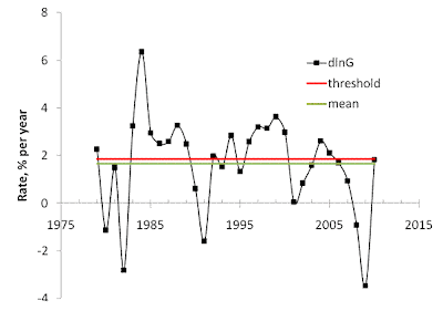
In (1), the rate of real GDP growth has a threshold of (0.866/0.465=) 1.86% per year for the rate of unemployment to be constant. When dlnG is larger than 1.86% per year the rate of unemployment in the U.S. starts to decrease. Figure 1 displays the evolution of dlnG since 1979. On average, the rate of growth was 1.65% per year, i.e. slightly lower than the threshold and the rate of unemployment has been increasing since 1979.
Figure 1. dlnG as a function of time. Also shown is the threshold of 1.86% per year, the mean growth rate of 1.65% per year.
When integrated between 1951 and t, equation (1) can be rewritten in the following form:
wt = 3.3 – 0.406ln[Gt/G1951] + 1.113(t-1951) + c1 , t<1979wt = w1978 – 0.465ln[Gt/G1978] + 0.866(t-1978) + c2 , t>1978 (2)
where wt is the predicted rate of unemployment. The intercept c1=c2≡0, as is clear for t=t0. Instead of using the continuous form (2), we calculate cumulative sums of the annual estimates of dlnG with appropriate initial conditions. By definition, the cumulative sum of the observdd du’s is the time series of the unemployment rate, ut. Figure 2 depicts the measured and observed curves.
The agreement is excellent and has been obtained by a formal statistical method. The integral form of the dynamic Okun’s law (2), i.e. wt=f(lnGt), is characterized by a standard error of 0.55% for the period between 1951 and 2010. The average rate of unemployment for the same period is 5.75% with the average annual increment of 1.1%. All in all, this is a very accurate model of unemployment. And this fact is the most intriguing one.
Figure 2. The observed and predicted rate of unemployment in the USA between 1951 and 2010.
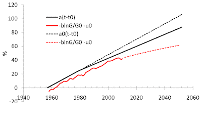
Our empirical model suggests a tangible shift in the slope and a significant change in the intercept around 1979. This is a very important finding. There are two terms in (2) which define the evolution of the unemployment rate: real economic growth, as expressed by the relative change in real GDP per capita, counteracts the positive linear time trend. Figure 3 depicts both components. The difference or the distance between a(t-t0) and –bln(Gt/G0)-u0 in Figure 3 is the rate of unemployment.
The importance of the structural break in 1979 is obvious when we extend the trend a(t-t0) observed before 1979. The distance would be much larger with the old trend after 1979, i.e. the rate of unemployment would have been also higher than that actually measured. If to extend the current time trend and the dependence on G through 2050 one can project the rate of unemployment as Figure 3 also depicts. Without a new structural break, the rate of unemployment in 2050 will be near 25%. This is grim news. It might happen that the U.S. is currently struggling through a transition to a new relation in (2) which will keep the rate of unemployment below 10%. In any case, the growth rate of real GDP per capita has to be much higher than 2% per year in order to reduce the current rate of unemployment to the level of 5%. Such a rate is not expected in the near future.
As an alternative, we have tried a logarithmic time trend instead of the linear one. The logarithmic trend easily follows from our model of economic growth which has an inertial component inversely proportional to the attained level of real GDP per capita:
dlnG/dt = 0.5dlnN9/dt + C/G (3)
where dlnN9/dt is the change rate of the number of 9-year-olds and C is an empirically estimated constant. The term C/G represents the inertial rate or growth, i.e. the rate of growth corresponding to no changes in the age pyramid. Figure 4 demonstrates the observed evolution of G since 1950 and gives two projections: a linear one with an annual increment C=$591.5 and an exponential growth following the trend before 2010. The deviation between these projections is fast and the next few years should distinguish between them. Figure 5 provides some examples of developed countries with linear trend in real GDP per capita.
We have introduced a similar trend term in the original Okun’s law and obtained:
dw/dt = A/Gt + bdlnG/dt (4)
By integrating (4) one obtains
wt = u0 + bln[Gt/G0] + A∫dt/Gt (5)
In the long run, the evolution of Gt is linear over time. Observations show that the change in the specific age population over the period of 50 and more years is negligibly small, ∫dlnN9/dt ~ 0. Then dlnG/Gdt=C/G and Gt=G0+C(t-t0). Therefore, both terms in (5) have a logarithmic trend in time and wt may vary around u0. For equation (2), these trends are different (linear and logarithmic) and wt must grow with time if there are no structural breaks. Figure 3 illustrates this divergence and the necessity of structural breaks.
We have checked the predictive power of (5) relative to (2) and found no improvement. On the contrary, (5) does not allow to describe the whole period between 1951 and 2010 with one constant A. Figure 6 depicts a model with A=28000 and b=-0.45. The model is very accurate between 1970 and 1990, overestimates the rate before 1970, and underestimates the observed rate after 2000.
Figure 3. The evolution of two components in (2) defining the unemployment rate.
Figure 4. The evolution of G over time with a projected linear trajectory for C=$591.5 and an exponential trajectory G=G0exp(0.0209t), where the exponent corresponds to that obtained for the period between 1950 and 2010.
Figure 5. Some examples of linear evolution of real GDP per capita in developed countries.
Figure 6. The observed rate of unemployment and that predicted by (5) with A=28000 and b=-0.45.
There is a fundamental concern about the excellent performance of Okun’s law in the U.S. The rate of unemployment is measured as a portion of labor force with the fluctuating rate of participation. This means that the sensitivity of unemployment to real economic growth, expressed by Okun’s law, does not depend on the rate of employment itself. Figure 7 compares the change in the rate of employment (the employment/population ratio), e, and the rate of unemployment. These two variables have been evolving in sync. Before 1980, the change in the rate of unemployment is relatively higher. After 1980, their amplitudes are very close.
Figure 7. The (negative) change in the rate of employment compared to the change in the rate of unemployment.
We have estimated a model similar to Okun’s law for the employment/population ratio, e:
de = 0.277dlnG – 0.457, t<1983
de = 0.496dlnG – 0.87, t>1982 (6)
Figure 8 compares the observed and predicted change in the employment/population ratio. Figure 9 shows the cumulative curves for the time series in Figure 8 and explains the structural break near 1982. The employment/population ratio grew from ~57% in 1982 and ~63% in 1989. This break also explains a similar break in the unemployment rate near 1980. The change in slope in (2) and (6) is rather similar: both the rate of employment and unemployment is more sensitive to the rate of change in GDP.
This is the effect we have already reported and modeled for the rate of participation in labor force, lt. To account for the effect of varying rate we introduced a factor, ft, exponentially depending on the difference between some reference rate, l0, and current rate, lt: ft=f0exp[g(lt-l0)], where f0 and g are empirical constants. The intuition behind the model is simple. The employment/population ratio and thus labor force increases with real GDP. When the rate of labor force participation undergoes a, say, 1% increase almost all new employees enter the workforce at the level of marginal personal income. Observations show that personal incomes are distributed exponentially in the low income range, i.e. the number of people with a given income decreases exponentially with increasing income. Accordingly, the input of the newcomers into the increasing GDP decreases exponentially with increasing labor force. Thus, the sensitivity of employment/population ratio to real GDP increases with the ratio.
This factor should be applied to Okun’s law as well. We will address this topic in the next post on employment.
Figure 8. The observed and predicted change in the employment/population ratio, de.
Figure 9. The cumulative curves for the observed and predicted change in the employment/population ratio, de.


0 komentar:
Post a Comment