Blame Demography for American's Weak Economic Growth

An article recently featured in The Economist explores the ways in which demographic changes have stifled economic growth. Many politicians have noticed the lagging economic growth rate following the greatest recession since WWII and are concerned that this may be the new norm. As The Economist explains, in the past three years the average growth rate stood at 2.2%, which is only slightly more than half the 4.2% averaged after the seven previous recessions. Part of the reason for the slower growth rate is that American's are facing unprecedented levels of debt and businesses are reluctant to spend, but changes in demography are also to blame for the slower recovery.
       The prime working ages are between 25 and 54 however the share of the population under 25 and above 54 continues to grow, causing a decline in overall labor-force participation rates. A few possible solutions are identified in the article to counteract this decline in labor force participation.  These include allowing more immigrants into America, reforming disability benefits to encourage those who are between the ages of 25 and 54 to go back to work, and raising the retirement age to keep workers in the labor force longer.

The Best Places for a Working Woman


According to The Economist, the United States ranks 12th out of 26 wealthy countries for a woman to work. The results were determined using five indicators including how many men and women who had secondary education, the percentage of women who participate in the labor force, the gap between the earnings of men and women, the proportion of women in high level positions, and the cost of child care compared to the average wage. 
 
New Zealand came in first place, followed by Norway, Sweden, Canada, and Australia. Although Finland placed 7th overall, it performed the best on measures regarding education. In Sweden, 78% of women participate in the labor force marking the highest rate out of all 26 countries. In Spain, the wage gap was only 6%, the lowest among all the countries. In contrast, Japan and South Korea were ranked quite low because there are few women in the country who hold high level senior positions.

More Chinese Women in Labor Force than Indian Women


Recent findings released by Gallupindicate that China’s female labor force participation rate (70%) is significantly greater than India’s (25%).  Not only are Indian women less likely to be present in their country’s labor force than Chinese women, women in India’s labor force are three times more likely to be unemployed (with an unemployment rate of 15%) than their Chinese counterparts (with an unemployment rate of 5%). Furthermore, women in China are nearly twice as likely to be employed full-time than women in India (21% verses 11%).  In addition, 53% of highly educated Chinese women reportedly hold a “good job” whereas only 17% of Indian women who received tertiary education maintain a “good job”.  There are also significant discrepancies in the literacy rates of Chinese females (91%) and the Indian females (50%).   In sum, Chinese women are much more likely to receive even a basic education than Indian women, and, among Chinese and Indian women who receive higher education, Chinese women are much more likely to find full-time employment. While the Chinese economy (with a 9% growth rate) is currently out-performing India’s economy, (with a 6.8% growth rate) China’s growth is expected to stall due to low fertility rates and an aging population. On the other hand, India’s population of working-aged citizens is expected to steadily increase until about 2030 and this can lead to major economic growth if India encourages greater female labor force participation.  

The rate of unemployment in the U.S. will fall to 6.2% by 2014

On March 1, 2012 we predicted (in a Seeking Alpha post) the rate of unemployment in the U.S. to fall down to 7.8% by 2013. The BLS announced 7.8% for September 2012. Here we present our basic model and predict the evolution of unemployment in 2013.

In 2006, we developed three individual empirical relationships between the rate of unemployment, u(t), price inflation, p(t), and the change rate of labour force, LF(t), in the United States. We also built a general relationship balancing all three variables simultaneously. Since measurement (including definition) errors in all three variables are independent it may so happen that they cancel each other (destructive interference) and the general relationship might have better statistical properties than the individual ones. For the USA, the best fit model for annual estimates was a follows:

u(t) = p(t-2.5) + 2.5dLF(t-5)/dtLF(t-5) + 0.0585 (1)

where inflation (CPI) leads unemployment by 2.5 years (30 months) and the change in labor force leads by 5 years (60 months). We have already postedon the performance of this model several times.

For the model in this post, we use monthly estimates of the headline CPI, u, and labor force, all reported by the US Bureau of Labor Statistics. The time lags are the same as in (1) but coefficients are different since we use month to month-a-year-ago rates of growth. We have also allowed for changing inflation coefficient. The best fit models for the period after 1978 are as follows:

u(t) = 0.63p(t-2.5) + 2.0dLF(t-5)/dtLF(t-5) + 0.07; between 1978 and 2003

u(t) = 0.90p(t-2.5) + 4.0dLF(t-5)/dtLF(t-5) + 0.30; after 2003

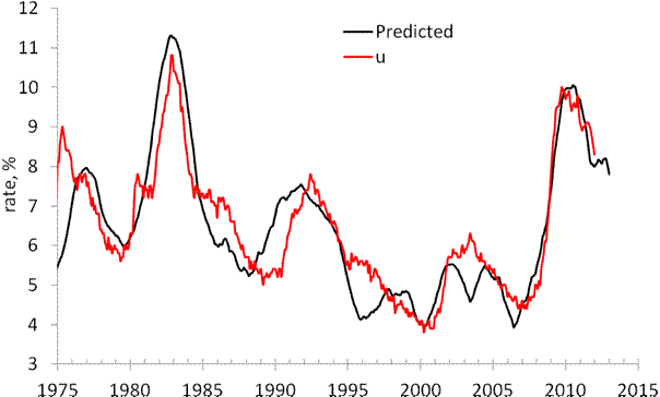
There is a structural break in 2003 which is needed to fit the predictions and observations in Figure 1. Due to strong fluctuations in monthly estimates of labor force and CPI we smoothed the predicted curve with MA(24).

The structural break in 2003 may be associated with the change of sensitivity of the rate of unemployment to the change of inflation and labor force. Alternatively, definitions of all three (or two) variables were revised around 2003, which is the year when new population controls were introduced by the BLS. The Census Bureau also reports major revisions to the Current Population Survey, where the estimates of labor force and unemployment are taken from.

On March 1, 2012 the monthly model predicted a drop from 8.3% in February to 7.8% by the end of 2012. Figure 1 depicts the original prediction (upper panel) and the observed fall in the rate of unemployment (lower panel). Figure 2 shows that the observed and predicted time series are well  correlated (Rsq.=0.81). This is a good statistical support to the model.

Figure 3 depicts the predicted rate of unemployment for the next 12 months. The model shows that the rate will fall to 6.2% by September 2013. For 105 observations since 2003, the modelling error is 0.4% with the precision of unemployment rate measurement of 0.2% (Census Bureau estimates in Technical Paper 66).
 
Hence, one may expect 6.2% [±0.4%].
 
 
Figure 1. Observed and predicted rate of unemployment in the USA as obtained in March and October 2012.


Figure 2.  Observed vs. predicted rate of unemployment between 1967 and 2012. The coefficient of determination   Rsq=0.81.


Figures 3. The predicted rate of unemployment. We expect the rate to fall down to 6.2% in September 2013.

7.8% unemployment was predicted in April 2012


In 2006, we developed three individual empirical relationships between the rate of unemployment, u(t), price inflation, p(t), and the change rate of labour force, LF(t), in the United States. We also built a general relationship balancing all three variables simultaneously. Since measurement (including definition) errors in all three variables are independent it may so happen that they cancel each other (destructive interference) and the general relationship might have better statistical properties than the individual ones. For the USA, the best fit model for annual estimates is a follows:

u(t) = p(t-2) + 2.5dLF(t-5)/dtLF(t-5) + 0.0585 (1)

where inflation (CPI) leads unemployment by 2 years and the change in labor force by 5 years. We have already postedon the performance of this model several times.

Here a model with monthly estimates of CPI, u, and labor force is presented. The time lags are the same as in (1) but coefficients are different since we use month to month a year ago rates of growth. We have also allowed for changing inflation coefficient. The best fit models for the period after 1978 are as follows:

u(t) = 0.63p(t-2) + 2.0dLF(t-5)/dtLF(t-5) + 0.07; between 1978 and 2003

u(t) = 0.90p(t-2) + 4.0dLF(t-5)/dtLF(t-5) + 0.30; after 2003

There is a structural break in 2003 which is needed to fit the predictions and observations in Figure 1. Due to strong fluctuations in monthly estimates of labor force and CPI we smoothed the predicted curve with MA(24). The rate of unemployment became more sensitive to the change of inflation and labor force. Alternatively, definitions of all three (or two) variables were revised around 2003, which is the year when new population controls were introduced by the BLS.

All in all, the monthly model predicts the observed rate of unemployment which has recently dropped to 8.3%. We expect the rate to fall further to the level of 7.8% by the end of 2012.


Figure 1. Observed and predicted rate of unemployment in the USA.

Japan - my scenario of consumer price fall was too optimistic

I've found a new projection of labor force in Japan between 2010 and 2050. It says that the rate of labor force participation will be decreasing together with the depopulation of Japan. This means that the level of labor force will be falling much faster than it was used in my recent prediction. Considering the multiplication factor of 1.4, the rate of CPI inflation will reach -1% per year on average in 2020. By 2050, it will reach almost 2% per year (1.89%). The overall drop in consumer prices will be more than 2/3 by 2050.  This fall will be accompanied by the decrease in real GDP at a rate of 1% per year and the debt rise to 500% of GDP.

Exploring Japan: on dismal perspectives of consumer prices

In this post, we continue to validate our predictions of the rate of consumer price inflation (CPI) in Japan by the estimate for 2011. The Japan Bureau of Statistics has estimated the rate of CPI inflation as -0.3%. Now we have an estimate of labour force for 2011 and are able to compare the observed and predicted  figures.  
We have been following inflation in Japan since 2005 when our first paper on the Japanese economy was published and covered the period through 2003. We have revisited inflation in Japan in 2010 and confirmed the predictions of deflation as expressed by the negative GDP deflator. In this blog, we also reported on deflation (both CPI and GDP deflator) several times.  
The case of Japan is the best illustration of our concept linking inflation to the change in labour force. (In a sense, all developed countries stay on the brink of deflation because of the threat of falling labour force.) Therefore we do not suggest the liquidity trap in Japan or any mistakes in monetary policy (inflation does not depend on monetary policy as our model shows.). The evolution of inflation is completely driven by the change in labour force. This is an unfortunate situation for Japan since the level of labour force can only fall in the long run due to the decreasing working age population.   
Previously, we carried out an estimation of empirical relationship between the change rate of labour force, dlnLF(t)/dt, and inflation, p(t).  
First, we test the existence of a link between inflation and labour force. Because of the structural (likely related to definition and measurement procedure) break in the 1980s, we have chosen the period after 1982 for linear regression. By varying the lag between the labour force and inflation one can obtain the best-fit coefficients for the prediction of CPI inflation, p(t),  according to the following relationship (updated with new data since 2009): 
p(t) = 1.39dlnLF(t-t0)/dt + 0.0004                                (1)
where the time lag t0=0 years; standard errors for both coefficients are shown in brackets.  Figure 1 (upper panel) depicts this best-fit case. (The period after 2003 is highlighted.) There is no time lag between the inflation series and the labour force change series in Japan. Free term in (1), defining the level of price inflation in the absence of labour force change, is statistically undistinguishable from zero.
A more precise and reliable method to compare observed and predicted inflation consists in the comparison of cumulative curves. Short-term oscillations and uncorrelated noise in data as induced by inaccurate measurements and the inevitable bias in all definitions should be smoothed out in cumulative curves. Any actual deviation between two cumulative curves persists in time if measured values are not matched by the defining relationship.
The predicted cumulative values shown in the lower panel of Figure 1 are very sensitive to the free term in (1). For Japan, the cumulative curves are characterized by complex shapes. There are periods of intensive inflation and a deflationary period. The labour force change, defining the predicted inflation curve, follows all the turns in the measured cumulative inflation.
One can conclude that relationship (1) is valid and the labour force change is the driving force of inflation. Statistically, the evolution of the overall level of consumer prices in Japan is fully defined by the change in labour force. Hence, no other variable or process can affect the change in price. Otherwise, the statistically reliable link would not exist.  
Having the projection of labour force borrowed from the National Institute of Population and Social Security Research, one can predict the future of CPI inflation in Japan. It will be decreasing to the level of -1% per year in 2050.  
Conclusion: invite immigrants and start a baby boom today! Otherwise, the level of consumer prices in 2050 will be a half of that of today.  
 
Figure 1. Measured inflation (CPI) and that predicted from the change rate of labour force. Upper panel:  Annual curves. Lower panel: Cumulative curves between 1982 and 2011. A good agreement between the cumulative curves illustrates the predictive power of our model.
 
Figure 2. Scatter plot: predicted vs. measured rate of CPI inflation.
Figure 3. Projection of the labour force evolution between 2005 and 2050.

Figure 4. The rate of CPI inflation in Japan through 2050.

Hispanics Represent Sizable Proportion of Labor Force Growth


The Pew Research Center reports that from 2010 to 2020, Hispanics are predicted to add 7.7 million jobs to the labor force.  This figure will account for 74% of the 10.5 million jobs expected to be added in total.  From 1990-2000, Hispanics added 36 percent of jobs to the workforce.  This percent jumped to 54 percent in the most recent decade of 2000-2010.  There are a couple factors involved in the high, and growing percentage of Hispanics added to the workforce.  Hispanics are growing in numbers due to a high birth rate and immigration.  On the other hand, the aging of non-Hispanic whites is predicted to diminish their numbers in the workforce.  In addition, a slightly higher percent of Hispanics, 67.5 percent, is actively searching for a job or is employed, compared to the national average of 64.7 percent.  Pew also notes that Hispanics are younger than other ethnicities, so their substantial contribution to the labor force should be expected to persist.

Modeling the change in unemployment rate: Canada, Australia and Spain

I continue model the change in unemployment rate as a linear function of the change rate  of real GDP per capita. (See my previous posts)

For Canada, I have estimated the following relation with a structural break in 1985
dlnG = -2.7du + 3.1, t<1995
dlnG = -2.7du + 1.2, t>1994
Figure 1 presents the observed dlnG curve and the scaled du, i.e. the change in GDP predicted from the change in the rate of unemployment.  The agreement is excellent, but both curves are volatile. I have smoothed them with MA(3).

For Spain, the result is really fantastic! the following relation is obtained with a structural break in 1987:
dlnG = -2.0du + 5, t<1987
dlnG = -0.8du + 2.1, t>1986

Figure 2 presents the observed and predicted dlnG. There might be another structural breal around 1970.

For Australia, the result might be not so exciting but is very good:
dlnG = -1.7du + 2.5, t<1995
dlnG = -3.0du + 1.3 t>1994

Figure 3 presents the observed and predicted curves smoothed with MA(3) and a structural breal in 1995. 
Figure 1. Annual growth rate of real GDP per capita, dlnG, and the scaled rate of unemployment, du. The lower panel shows the curves smoothed with MA(3)


Figure 2. Same as in Figure 1 for Spain .

Figure 3. Same as in Figure 1 for Australia


Bravo, Krugman!

A month ago I presented a graph linking the growth rate of real GDP per capita and the rate of unemployment. Figure 1 is borrowed from this post and shows that one can expect the rate of unemployment to  fall fast in the second half of 2011.

Figure 1. The annual change rate of real GDP, dlnGDP/dt, and the scaled rate of unemployment, UE.
Paul Krugman has modified this graph in order to prove that the current  rate of unemployment is a direct consequence of slow real growth. He plotted the change in unemployment rate against the change rate of real GDP.  In his scatter plot, correlation was very high.  I decided to repeat his result using GDP per capita instead of the overall GDP, which is a biased measure of growth in econometric assessments.  The only thing I have to say:
Bravo, Krugman!
This is almost the best economic graph I have ever seen. Figure 2 presents it in my interpretation and shows that the change in unemployment rate, du, almost coincides with the change rate of GDP per capita, dlnG. In Figure 2, we have scaled the du with the following relationship:
dlnG = -2.37du+2.25
or
du= -0.42 dlnG + 0.95
Figure 3 presents results of regression: Rsq.=0.81. For the scaled du, the slope is 1.0.

However, the current fall in the rate of unemployment exceeds the predicted one. Somehow, the sensitivity of the du to dlnG becomes lower after 2000, and the slope of -1.6 and the intercept of 2.1 better describe the link.  For these values of slope and intercept, the rate of real economic growth, dlnG, should be ~2% per year for the rate unemployment retained at 9.6%. For the rate of unemployment to fall, one needs the real growth rate above 2% per year.
Figure 1 looks a bit biased. We have also to reconsider this post on unemployment as based on the change in labor force, which predicted the rate of unemployment around 8% in 2012.
Figure 2. Annual growth rate of real GDP per capita, dlnG, and the scaled rate of unemployment, du.

Figure 3. Scatter plot of the curves in Figure 2 and linear regression.


Figure 4. Same as in Figure 2 with the slope -1.5 and intercept +2.0 for the period after 1995.

Is the employment situation really disappointing? II

This post almost completely repeats our post on employment situation a month ago.
The Bureau of Labor Statistics has published an “Employment Situation Summary” for June. The nonfarm payroll employment has increased by 18,000 (establishment data). The number of employed in the U.S. has decreased by 445,000; from 139,779,000 to 139,334,000 (household data).  As in May 2011, these low numbers have come as a surprise for many experts, who expected 105,000 for the nonfarm payroll employment in June.

We have already demonstrated that the level of labor force in the U.S. has been experiencing an unprecedented fall since 2008. Figure 1 reminds us that the reason for the fall is not the current financial crisis and recession but rather a new trend in the rate of labor force participation, LFP. This is not a short- or mid-term transient process but the change in the long-term tendency. The LFP had been growing between 1955 and 2000, when it reached its peak. One can consider 2001 as a pivot point manifesting a fundamental change in the labor market behavior in the U.S. It is worth noting that the change in LFP behaviour started ten years ago, not in 2008. (The reader might be interested in the explanation of this phenomenon. We had accurately predicted the 2010/2011 fall in the LFP many years before it happened.)

As a result of the new long-term tendency, one should not expect the same pace of employment growth as it was between 1960 and 2000. In addition to the fundamental shift in the secular LFP evolution, one should not forget another source of employment growth – the level of working age population. Figure 2 depicts monthly increments of the working age population, i.e. 16 years old and over.  One can clearly see that the influx of the population has been decelerating since 2000 as well. The deep negative corrections in Figure 2 are associated with annual revisions to population controls. It is not wise to wait that the growth in employment will exceed the influx of working age population in the situation with the falling LFP.    

It is important that even decreasing unemployment can not compensate the effects of LFP and population. Figure 3 shows the evolution of monthly increments in employment, E, after 2003 with MA(12). One should not expect that E will be growing at a pace which was considered as a healthy one before 2000 any time soon. As a month before we can conclude that the today’s BLS figures are not disappointing. Really disappointing is the unjustified expectation of any large increase in the U.S. employment.  


Figure 1. Measured LFP in the U.S.


Figure 2. Monthly increment in working age popualtion (16 years of age and over) in the U.S.


Figure 3. Monthly increment of employment in the US with its MA(12).

An open letter to the U.S. Bureau of Labor Statistics

Five years ago I published a paper on the link between inflation and labor force in the U.S. There was one stupid problem with the estimates of labor force level provided by the BLS. They competely  ignored the changes in so called population controls after decennial censuses. Briefly, any census reveals the difference between projected and directly enumerated populations. The former figures are projected from the previous census using estimated birth and death rates and net immigration. After any census, this difference called "the error of closure"  is proportionally distributed by the U.S. Census Bureau  (CB) over the previous decade. This prodecure makes all population time series reported by the CB smooth.

The BLS does not address this problem at all. Therefore, its labor force time series has several "bumps" of a million an more people per one month. One should not use this time series as it is in statistical of econometric assessments.  I had to redistribute all known bumps back into their  past and obtained relatively smooth time series. This simple procedure did not work well in 1991 and additional investigation was needed to recover the reason of ~1,000,000 step in the labor force series.

Recently, I have found a paper written by Marisa Di Natale "Creating Comparability in CPS Employment Series"  from the BLS (no publication date is specified). The author used the same method of the error of closure redistribution. It is a good paper with a simple but correct methodology. But do not believe it. The original time series has not been smoothed. I downloaded the most recent version of labor force time series )July 1, 2011) and found no changes in 1991 and 2001. Same sharp spikes:

Figure. Monthly increment of labor force in the U.S.


Conclusion: Do not trust BLS!

On the slow growth of working age population

There is a discussion on the Seeking Alpha of my post on the last Employment Situation Summary issued by the BLS several days ago. Lee Adler asked about the evolution of working age population, WAP, in the U.S. during the past 50 years. This question has arisen because I had shown only the last ten years in the post. These were the years of a steady decrease in the annual increment of the working age population, which is defined as the number of people of 16 years of age and over.  Lee is right; the annual increment has two peaks - in the 1970s and between 1998 and 2003 as Figure 1 shows.  During the 1980s and 1990s, the increment was at the level of 2,200,000 per year, and in the 2000s it fell from 3,000,000 and more per year to ~2,000,000 per year in 2008 and 2009. One should not trust the peaks in 2000 and 2003. These are caused by one-sided revisions of the total population after the 2000 census. The numbers were corrected after 2000 and 2003 but not before what created severe steps in the WAP.
Figure 2 depicts the evolution of the change rate of the WAP, dWAP/WAPdt or dlnWAP/dt. This is to show that in relative terms (the rate of unemployment and employment-population ratio are defined in relative terms) the current growth of the WAP is not fast from the historical point of view. The 2008 through 2010 values are the smallest since the early 1950s when the aftermaths of the Great Depression and WWII were the most painful. Thus, the current decrease in the growth rate of working age population is one of the reasons behind the slow employment recovery.

Figure 1. Annual increment of the working age population (black line) and its 5-year moving average (red line).

Figure 2. The rate of growth of the working age population (black line) and its 5-year moving average (red line).

Blog Archive